Carbon accounting methods require the management of different data sources and their combination into aggregated data. Doing so in real-time is another challenge in itself. In this tutorial, we learn how to use plug-and-play solutions by Confluent Cloud to perform these tasks more easily. You will set up and integrate data from a SQL¹ database, an event producer and an API² for carbon footprint calculation. Afterward, you will merge this data to calculate emission metrics, that you can display in a Power BI dashboard.

Our toolset

Most of the upcoming activities will be accomplished within the cloud services of Microsoft, namely Confluent Cloud for MS Azure and Power BI Service. The tutorial “How to build your first event streaming dashboard” introduced these platform solutions that are easily accessible through your browser. Please visit the post if you have not yet worked with these tools to get started. It’s fine if you don’t have expertise and don’t worry about paying money for your experiments. In this post you will also find enough training material and instructions on how to set up free trial accounts.

This time around we will not utilize the Datagen Source Connector by Confluent to simulate incoming data from an Apache Kafka producer. Now it’s time to build our own producer using the Python code I prepared so you can run it locally on your computer with a Jupyter Notebook. For this part it is helpful to have basic knowledge of the Python programming language. However, the setup and execution is kept simple enough that you can do without it.

Using Confluent does not mean that we have to limit ourselves to getting data from an event producer. With a set of API connectors, we can access data from static sources such as SQL databases or retrieve data from more dynamic sources such as external APIs. To follow best practices for managing ever-changing inputs and outputs, we will use Confluent’s integrated schema registry. Background information on both technologies can be found in the related context post.

Since we need to merge our heterogeneous data Kafka-style in real-time, we will also use the ksqlDB service by Confluent. Basic knowledge of SQL is helpful when we work with ksqlDB. But as always, you will be able to complete all steps simply by copying and running the code snippets I provide. Let’s take a closer look at the technologies underlying both Confluent Schema Registry and ksqlDB.

Introduction to fundamental concepts

1) Basics of Confluent Schema Registry

In IT, data (models) are usually formalized and enforced by schemas. Data exchange via APIs can also benefit from schemas if the sending and receiving sides agree on a standard. This is especially true for the phenomenon of schema evolution. The term describes the continuous change of data over time, as new information and capabilities on whatever side require constant adaptation of the schema. This is usually the reason why we want to ensure backward compatibility with exchanged data objects. Imagine a sender updates its data model, while the recipients do not want to accept this change. If we have a version control system that allows backward compatibility, we can update the schema with a new version while older versions are still supported.

This capability is provided by schema registry tools such as Confluent Schema Registry. However, you can also implement schema validation and versioning using other formats, frameworks, and tools (see related context post). Confluent Schema Registry enables the centralized and transparent management of schemas. This not only facilitates collaboration and schema evolution, but can also serve as a layer of protection against unwanted changes. The schema registry acts as a principal where new schemas or schema changes must be properly registered. Once stored, existing schemas are sourced from the registry to validate incoming and outgoing messages. The figure below illustrates this validation process while including the integral role serializers and deserializers play.

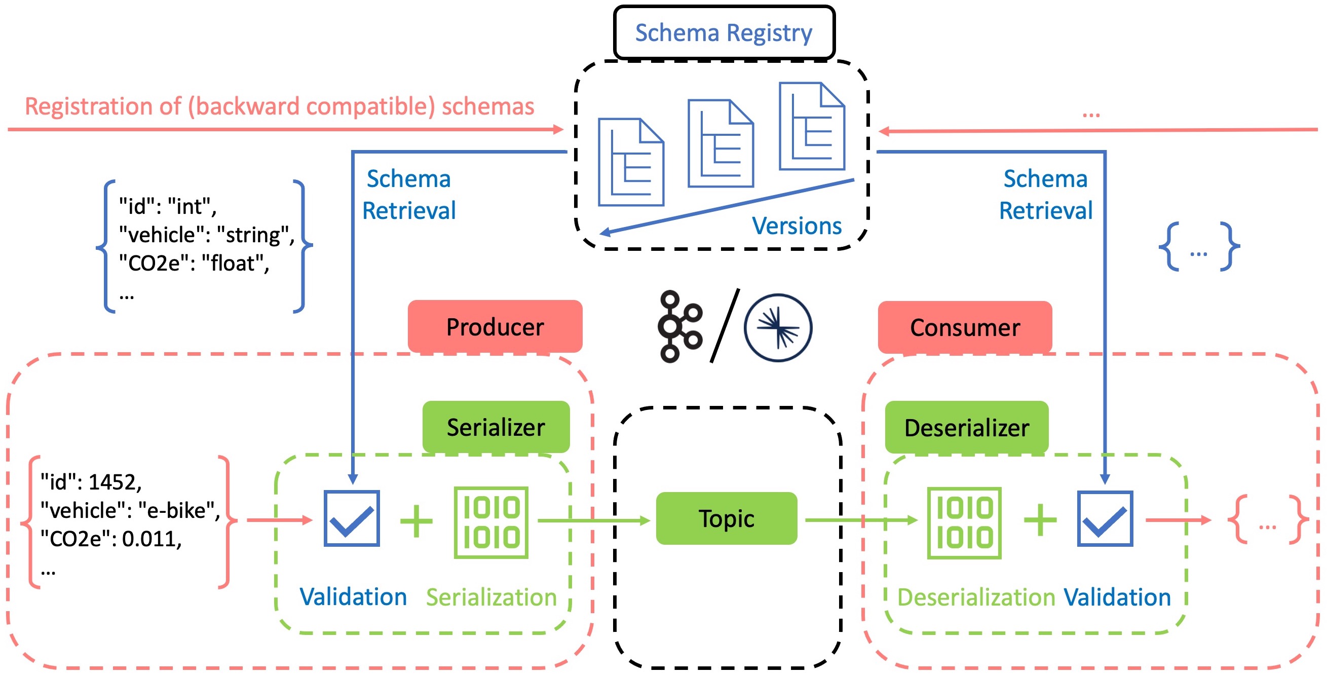
Fast and efficient data exchange is a strength of Apache Kafka and is made possible by the binary format used internally. This significantly reduces memory and computing resources for storage and distribution. Consequently, producers must encode their messages into this format using serializers, while consumers must decode them using deserializers. During this process, it is convenient to use schemas as encoding/decoding instructions and verify that the outgoing/incoming messages conform to the specifications. In JSON³-based serialization formats like AVRO⁴, we can specify the structure, keys and values of messages. Serialization/ Deserialization (SerDe) fails if the input/output functions try to subvert the agreed standard by making unknown changes. If you want to acquire more in-depth and practical knowledge about the Schema Registry, I can recommend the training material from Confluent.

2) Basics of ksqlDB

Many know and appreciate the simplicity of SQL when it comes to data aggregation in relational databases. To process data from Kafka topics using familiar SQL commands, Confluent has developed ksqlDB, which uses an ANSI SQL dialect⁵. This makes it a powerful tool for event streaming scenarios where continuous transformations are required. Migration of existing processing logic from systems that use a SQL dialect is also made easier. Note that there are other stream processing frameworks with similar capabilities on the market. The related context post lists comparable solutions and explains the importance of language standards such as ANSI SQL.

To enable scalable and robust stream processing, ksqlDB runs in a compute cluster separate from the Apache Kafka clusters. However, Kafka topics continue to be used as storage for the two fundamental constructs of ksqlDB, streams and tables. Streams embody the typical event-driven data that is constantly and rapidly changing. Tables, on the other hand, represent a collection of state-related records. Like tables in the relational sense, they contain only the most recent value for a primary key. The ability to use sequential commands to create streams and join them with other streams or tables makes ksqlDB very versatile. In the next steps of the tutorial, we will learn about some practical examples. For now, I’ll leave you with some additional training material on ksqlDB.

Real-time carbon accounting for an e-bike rental service

A previous context post presented the benefits of event streaming in scenarios where high data throughput is required. For example, in cases with many customer interactions. The e-bike rental use case in the related context post expresses such a need, as timely carbon accounting should be performed for each service use. At the end of this post you will find an overview of the initial situation, before we move on to the actual implementation of the technologies discussed. If you need a brief introduction to emissions calculation with CO2e⁶ in the context of carbon accounting, you will find a section on this in part 1 of the related post.

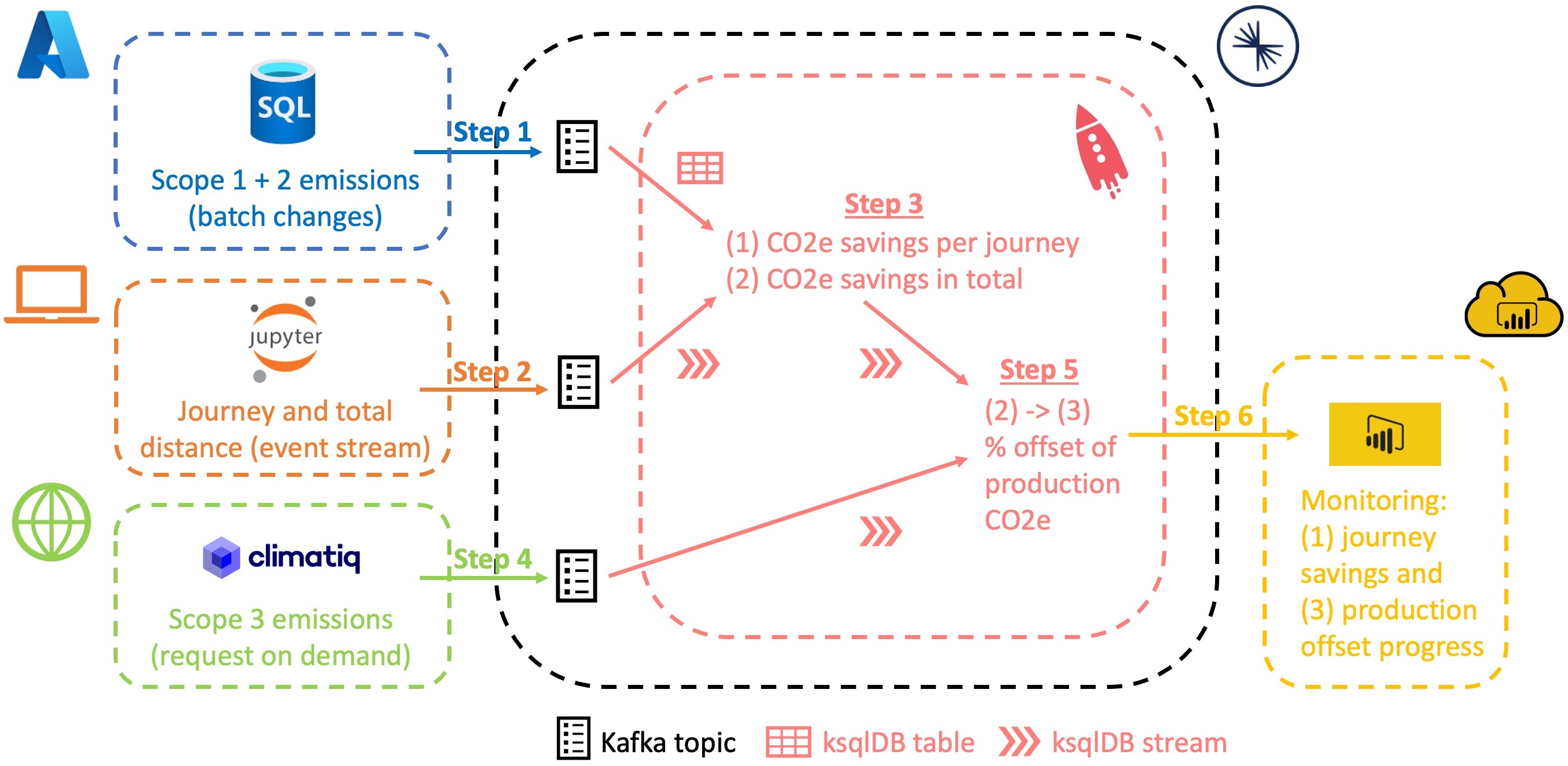
We are now addressing the e-bike rental scenario by building a prototype that can process simulated enterprise data and even real emissions data. Our first goal is to calculate the CO2e savings that each journey generates. Finally, we report the percentage that indicates progress toward the break-even point of the e-bike’s production emissions, i.e., progress toward offsetting production CO2e.

For technical preparation, you should refer to the points in the Our toolset section so that you can start directly with step 1 of this tutorial. Please also note that the steps explained in detail in the previous tutorial are not repeated. However, you can see how each action is performed in the videos at the beginning of each section. Many steps show code snippets that you need to enter into the respective tooling. You will find a description of each command as comments in the code.

Step 1: Azure SQL DB and connector setup

To simulate the operation of an e-bike rental business, we need suitable data. This scenario was not chosen by chance, because Azure provides a pre-built database template for training purposes on this topic. We can modify the Adventure Works template for our purposes by adding data of an e-bike rental business to the fictitious bike store. Let’s imagine that Adventure Works is a climate-conscious company that has implemented a carbon accounting (CA) system in the background to track its Scope 1 and Scope 2 emissions. It breaks down emissions to the product/service level, i.e., average CO2e levels per kilometer (km) driven for each customer trip.

We now assume that the CA engine regularly updates the following two values for each e-bike model: Average Scope 1 CO2e values per km (emissions from storage facilities, transport of e-bikes to sites, etc.) and average Scope 2 CO2e values per km (electricity consumption of e-bikes). According to the assumptions in the related context post, Scope 2 values will be negative because Adventure Works uses renewable energy credits or generates its own electricity renewably. The existing database template contains data for the three regular bicycle categories of road bike, mountain bike, and touring bike. We assume that the most expensive configuration of these categories in the range of $1481.94 to $2171.29 is the purchase price for e-bike procurement. Another simplifying assumption is that average electricity consumption ranges from 0.011 CO2e to 0.021 CO2e, with the touring bike using a typical e-assist motor, while the road bike supports up to 100% motorized propulsion.

Let’s set up the aforementioned database. To do this, log in to your Azure workspace and follow these steps to create a new Azure SQL instance:

• Select a single SQL database as the deployment option.
• Enter the name of your resource group (RG) and subscription. Select a new database name such as “adventure_db”.
• Create a new server (e.g. “unique-name-server”) within your RG location and select the SQL server authentication method. Create your admin credentials (e.g. “adventure_dev”) and store them securely.
• Keep the compute and locally redundant backup settings for cheap training purposes.
• Choose a public endpoint connection. In the firewall rules, select Allow Azure services and resources and add the current client IP address. Usually, it is best practice to set up a virtual network and build private link connections between Azure resources. But for simplified training purposes, we won’t go into networking in this tutorial. Never use these settings in a productive environment due to their increased vulnerability.
• In the additional settings, select Sample as the data source.

After successful deployment, navigate to the query editor of your new SQL database and log in. There you can view and edit your data using the following SQL Server queries:

/*Creating a new table BikeEmissions that has all the 
relevant columns we need*/
select t1.ProductCategoryID, t1."Name", t1.AVGcost, 
t1.CO2e_km_scope1, t1.CO2e_km_scope2
into BikeEmissions

/*Inserting exsiting product information for all three 
bike categories into BikeEmissions, while adding new values 
like names and CO2e estimates.*/
from
(select ProductCategoryID,
'Road E-Bike' as "Name",
cast((round(max(StandardCost),2)) as float) as AVGcost,
0.005 as CO2e_km_scope1,
-0.021 as CO2e_km_scope2
from [SalesLT].[Product]
where ProductCategoryID = 6
group by ProductCategoryID

union

select ProductCategoryID,
'Mountain E-Bike' as "Name",
cast((round(max(StandardCost),2)) as float) as AVGcost,
0.005 as CO2e_km_scope1,
-0.016 as CO2e_km_scope2
from [SalesLT].[Product]
where ProductCategoryID = 5
group by ProductCategoryID

union

select ProductCategoryID,
'Touring E-Bike' as "Name",
cast((round(max(StandardCost),2)) as float) as AVGcost,
0.005 as CO2e_km_scope1,
-0.011 as CO2e_km_scope2
from [SalesLT].[Product]
where ProductCategoryID = 7
group by ProductCategoryID) t1


/*Making sure the primary key ProductCategoryID,  
is not nullable as required by Kafka later on.*/
alter table [dbo].[BikeEmissions]
alter column ProductCategoryID int NOT NULL

After executing all three instructions, we have our basic Scope 1 and 2 data for each of the three bike categories. Now we can feed this data into a Kafka topic within Confluent Cloud using a fully managed plug-and-play API connector. Navigate to your current cluster, click add connector and look for the Microsoft SQL Server Source connector. We’ll choose a name like “scope1and2.” for the new topic to write the SQL DB data to. After creating a new access key or using an existing one, we add the following authentication settings:

• The host/server URL⁷ from the Azure DB settings.
• 1433 as the port (common Azure setting).
• The admin credentials we created earlier for the SQL DB.
• The name of the database (e.g. “adventure_db”).
• 120000 (milliseconds) as the poll interval, since an hourly database update should be sufficient for now.

In the configuration settings, we add:

• The name of the target table, in our case BikeEmissions.
• AVRO as our preferred record value. This will automatically create a schema in our schema registry that matches the SQL data we entered.
• Incrementing as the mode and ProductCategoryID as the incrementing column name. This tells Kafka how to distinguish new rows.
• best_fit_eager_double for Numeric Mapping to correctly transfer floating point entries like our CO2e values.
• In the Transforms section we add two SMTs: copyFieldToKey (as a name) with ValueToKey as TransformType and extractKeyFromStruct (as a name) with ExtractField$Key. Both of them search for ProductCategoryID as event key. To get to know more about the meaning of the event key visit the previous tutorial. Once the connector is implemented, we can see the SQL data read in our corresponding topic.

Step 2: Setting up a local producer with Python

The following actions are performed in a locally running Jupyter notebook with a Python virtual environment. If you don’t have one yet, you need a Python installation on your machine. Follow the instructions of the Jupyter project to install Python with the Anaconda distribution. Before we can start working, you should clone or download my project repository. After this follow the instructions in the README file to complete the prerequisites.

To enable the connection from our local host to Confluent, we need to edit the configuration file of our project. Navigate to the Client tab of our cluster in Confluent and create an API key for the cluster and schema registry. We can then simply copy the template on the right and replace the contents of the python.properties file in the confluent folder with this one. Edit the config.py file to contain the same credentials. Then create a new topic with a name like “tracking_events” and 1 partition.

After running the notebook, you have generated some tracking data on a topic that matches a backward compatible schema. We can rerun the data generation snippets and produce more data anytime we want, simulating customer interaction as needed. Remember that schemas and SerDe⁸ functions protect against unwanted changes to our data, and you can test this as well. If you want to learn more about the Python client for Confluent have a look at this tutorial.

Step 3: ksqlDB setup and Stream-Table join

Now we want to merge the CO2e values of Scope 1 and 2 with the corresponding tracking data. To do this, we need to get a ksqlDB instance running. Navigate to the ksqlDB section of your current confluent cluster and select Create cluster myself. Decide on the default settings with global access. Deployment may take a while. Note that running a ksqlDB cluster is one of the more expensive operations in Confluent Cloud (about 0.2€/h). Therefore, make sure you document important query commands for replication and delete the cluster as soon as you finish your tests. Unfortunately, there is no pause option at the moment.

After provisioning, we will find an editor in the navigation area of the new cluster. Here we can enter the following KSQL commands to create a data stream about the CO2e values per journey and the bikes travel distance in total. You can check the actual data with common SELECT queries. Just make sure you set the auto.offset.reset property to Earliest and wait a moment so you can see the historical data.

/*During the initial stream creation we need to access the nested 
elements of messages with ARRAY and STRUCT commands native to Kafka 
and ksqlDB. For more information see https://www.confluent.io/blog/data-wrangling-apache-kafka-ksql/ */
CREATE STREAM TRACKING_EVENTS(
	id BIGINT,
    customer_id BIGINT,
    date_time BIGINT,
    measurement_list ARRAY<STRUCT<vehicle_id BIGINT,
					    product_id BIGINT,
					    journey_km DOUBLE,
					    total_km DOUBLE>>
  ) WITH (
    KAFKA_TOPIC = 'tracking_events',
    VALUE_FORMAT = 'AVRO',
    PARTITIONS = 1
  );

/*We flatten this nested data with the 'explode' function of ksqlDB, 
preparing for the upcoming Stream-Table join. For more information
see https://docs.ksqldb.io/en/latest/developer-guide/ksqldb-reference/table-functions/#explode */ 
CREATE STREAM FLATTENED_EVENTS AS
	SELECT
		id AS event_id,
		customer_id,
		TIMESTAMPTOSTRING((date_time*1000), 'yyyy-MM-dd HH:mm:ss') as date_time,
		explode(measurement_list) as measurement
	FROM
		TRACKING_EVENTS;

/*Extraction and casting of flattened data*/	
CREATE STREAM EVENTS_BY_PRODUCT 
WITH ( PARTITIONS = 1, KAFKA_TOPIC = 'events_by_products', VALUE_FORMAT = 'AVRO') AS
	SELECT
	    event_id,
	    customer_id,
	    date_time,
	    CAST(measurement->vehicle_id as VARCHAR) as vehicle_id,
	    CAST(measurement->product_id as VARCHAR) as product_id,
	    measurement->journey_km as journey_km,
	    measurement->total_km as total_km
	FROM  
		FLATTENED_EVENTS;

/*Creating a ksqlDB table for our scope 1 and 2 data as it 
is state-related.*/
CREATE TABLE BIKE_DATA (ID VARCHAR PRIMARY KEY)
WITH (KAFKA_TOPIC='scope1and2.BikeEmissions', VALUE_FORMAT='AVRO', PARTITIONS=1);

/*Stream-Table join on the common product id (of the 3 bike types) with 
a calculation of CO2e values per journey and per total travel distance.
For more information see https://docs.ksqldb.io/en/latest/developer-guide/joins/join-streams-and-tables/ */
CREATE STREAM EVENTS_W_SCOPE_1_2 AS SELECT
  ebp.event_id,
  ebp.customer_id,
  ebp.date_time,
  ebp.vehicle_id,
  ebp.product_id,
  ((bd.CO2e_km_scope1 + bd.CO2e_km_scope2) * ebp.journey_km) as journey_CO2e_1_2,
  ((bd.CO2e_km_scope1 + bd.CO2e_km_scope2) * ebp.total_km) as total_CO2e_1_2,
  bd.AVGcost
FROM EVENTS_BY_PRODUCT ebp
LEFT JOIN BIKE_DATA bd ON ebp.product_id = bd.ID
EMIT CHANGES;

Step 4: API connection to Climatiq

So far, we have been working with fictitious data to simulate the emissions tracking of an e-bike rental service. Now we want to bring some real-world emissions data into the mix using an external API service. We will use Climatiq as the provider of Scope 3 data on the emissions of e-bike production. Climatiq provides a range of emission factors from various sources. For our purpose, we can use the Motorcycle/bicycle and parts activity from the US Environmental Protection Agency (EPA) calculations. Due to its broad scope and expenditure-based approach (CO2e/USD), we can use it for our e-bike scenario.

For this purpose, we will query the Climatiq API with information about the average price for each of our three e-bike categories. To get free access to the API with a limit of 250 calls per month, sign up for the Community Plan. If you need a trial period with a higher number of requests, please contact the Climatiq team via the contact form. In the course of preparing for the tutorial, I had a very positive experience with it. The contact persons are very friendly and can answer specific questions about datasets and licenses.

Once signed up, go to your Climatiq dashboard to create and save the API key that we need for authentication. Then we access the Data Explorer and look for the mentioned activity. Open the Show API Code Snippet feature window. Leave it open, because in the next steps we will copy the two parts --url and --data. Now you can go to Confluent Cloud and prepare our integration by creating a new topic with a name like “scope3.Climatiq” and 1 partition. You can skip the schema creation part as this will be done automatically during set up of the connector.

Navigate to the Connectors tab and select the desired HTTP Source Connector ⁹. Edit the settings here as follows:

• Create a new Kafka API key or paste an existing key
• Enter the name of the previously created topic (e.g. “scope3.Climatiq”)
• Paste the Climatiq API URL that we copied from the climatiq API code fragments section earlier. Next, select bearer as the endpoint authentication type and enter the bearer token (API key) previously generated by Climatiq
• Select POST as the HTTP request method
• Briefly copy the --data body from the cimatiq template into a text editor and change the value of the money key to ${entityName}. This parameter will be used by the connector to insert our respective bike price values. Enter the edited string in the HTTP request body field.
• Select 0 as the HTTP initial offset and 120000 as the request interval. We will only request the required emission data once and will not need to update it frequently for this use case. Please keep this number high if you want to keep your costs and the number of API requests low during testing.
• Enter the e-bike price values 1481.94,1912.15 and 2171.29 separately in the Entity Name field. The connector iterates through these values to insert them into the request body.
• Select 1 for the maximum number of retries to stop the connector early in case of connection problems
• Select true for SSL Enabled
• AVRO should be the format of the output record so we can automatically create a matching schema.
• One task is sufficient. Click Next and start the connector.

Once connected, three entries, one for each bike category, will be displayed in our new topic. You can keep the connector running to update this information every hour. However, since the HTTP connector is one of the more expensive Confluent resources ($0.3/hr) and we already have the information we need, it can be paused or deleted. Remember to set the retention period for your new topic long enough so that the data is not lost due to a scheduled deletion. If you are concerned about the number of Climatiq requests remaining, you can view your current API usage in the Climatiq dashboard settings.

Step 5: Final Stream-Stream join

With the sample data from all three sources now integrated into Kafka topics, we can proceed with the final aggregation task. The Scope 3 CO2e values from Climatiq now allow us to calculate the offset progress (in %) towards breaking even on production emissions for each bike. Run the following statements in the editor of our running ksqlDB cluster.

/*Stream creation and access to nested elements as shown before. */
CREATE STREAM SCOPE3_DATA (
	emission_factor STRUCT<name VARCHAR>,
    activity_data STRUCT<activity_value DOUBLE>,
    co2e DOUBLE
  ) WITH (
    KAFKA_TOPIC = 'scope3.Climatiq',
    VALUE_FORMAT = 'AVRO',
    PARTITIONS = 1
  );

/*Flattening as shown before and creation of a unique composite_key 
through concatination as we did not have an event key yet.*/
CREATE STREAM SCOPE3_DATA_FLAT WITH ( PARTITIONS = 1, KAFKA_TOPIC = 'scope3_data_flat', VALUE_FORMAT = 'AVRO' ) AS 
    SELECT
		CONCAT(CAST(emission_factor->name AS VARCHAR), '-', CAST(activity_data->activity_value AS VARCHAR) ) AS composite_key,
		activity_data->activity_value as dollar,
		co2e
	FROM  
		SCOPE3_DATA;

/*Stream-Stream join on the average purchase price to calculate 
the break even progress with scope 1,2 and 3 CO2e values. 
Adding 100 as the maximum percentage goal. Stream-Stream joins 
require you to set a WITHIN clause for matching records in a 
specified time interval. For more information see https://docs.ksqldb.io/en/latest/developer-guide/joins/join-streams-and-tables/ */
CREATE STREAM EVENTS_W_SCOPE3 AS SELECT 
	e12.event_id,
	e12.customer_id,
	e12.date_time,
	e12.vehicle_id,
	e12.product_id,
	e12.journey_CO2e_1_2,
	(ABS(e12.total_CO2e_1_2 / s3.co2e)*100) as percent_break_even,
	100 as max_break_even
	FROM EVENTS_W_SCOPE_1_2 e12 JOIN SCOPE3_DATA_FLAT s3 
	WITHIN 3 HOURS GRACE PERIOD 12 HOUR
	ON e12.AVGcost = s3.dollar
	PARTITION BY e12.event_id;

Step 6: Push to Power BI and visualization

Adventure Works rental customers could now receive notifications about their CO2e savings for each ride and the progress it made toward offsetting their bikes production emissions. You could call up the Jupyter Notebook and use the Python consumer client to simulate this case. But to make things more descriptive, we visualize our results in Power BI Service. This way, we can share the processed information with another audience, such as an internal carbon accounting team.

Streaming data in Power BI is done via an HTTP Sink Connector as shown in the previous tutorial. There you will find a detailed description of the necessary settings or you simply follow the steps in the video above. We can now use the looping feature of our Jupyter Notebook code to continuously produce events that result in continuous output of CO2e metrics. One important change from the previous tutorial is that we will no longer use the “Historic data analysis” setting of the streaming dataset. This allows for a more powerful ingress frequency since we only need the most recent data. The limitation of using Power BI streaming data sets, is that we cannot process this real-time data in Power BI. Additional filtering, aggregation and other processing would need to be done in ksqlDB. However, this should not be the main issue as it is best practice to place transformative tasks near the data storage and distribution backend anyway.

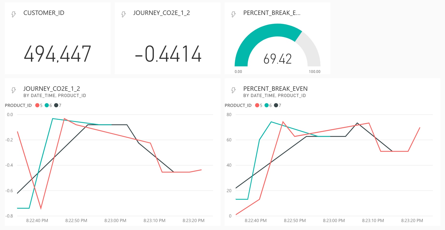
After establishing a push connection to a streaming dataset in Power BI, we can visualize selected values in a new dashboard. To track current savings and progress values, a line chart is helpful. Grouping data by product type can also provide good insights into the current status of emissions reduction linked to the e-bike fleet. You can play with other visualizations and edit the code provided so far to customize the use case to your liking. So far though, congratulations on completing this comprehensive tutorial and I look forward to any feedback you have.

¹ Structured Query Language (SQL) - relational database language
² Application Programming Interface (API)
³ JavaScript Object Notation (JSON) - data exchange format
⁴ Apache Avro, here just AVRO - serialization format with schema capabilities
⁵ American National Standards Institute SQL (ANSI SQL) - standard for SQL
⁶ Carbon dioxide equivalent (CO2e) - unit that summarizes climat impact of different greenhouse gases
⁷ Uniform Resource Locator (URL) - identifier that locates a resource on the Internet
⁸ Serializer/Deserializer (SerDe) - components that convert data objects into a (binary) format for storage or transportation
⁹ Hypertext Transfer Protocol (HTTP) - application layer protocol for the Internet